2d Temporal Model: Tutorial on real data

library(ETAS.inlabru)
library(ggplot2)

# Increase/decrease num.cores if you have more/fewer cores on your computer.
# future::multisession works on both Windows, MacOS, and Linux
num.cores <- 2
future::plan(future::multisession, workers = num.cores)
INLA::inla.setOption(num.threads = num.cores)
# To deactivate parallelism, run
#   future::plan(future::sequential)
#   INLA::inla.setOption(num.threads = 1)

Introduction to ETAS model

In this tutorial, we show how to use the ETAS.inlabru R-package to fit a temporal ETAS model on real earthquakes data. The tutorial shows how to prepare the data, how to fit a model, how to retrieve the posterior distribution of the parameters and the posterior distribution of other quantities of interest, how to generate synthetic catalogues from the fitted model, and how to produce forecasts of seismicity.

The Epidemic-Type Aftershock Sequence (ETAS) model belongs to the family of Hawkes (or ) point processes. The temporal Hawkes process is a point process model with conditional intensity given by

$\lambda(t | \mathcal H_t) = \mu + \sum_{t_h \in \mathcal H_t} g(t- t_h)$ where $\mathcal H_t$ is the history of the process up to time $t$ . Generally speaking $\mathcal H_t$ contains all the events occurred before $t$ . The quantity $\mu > 0$ is usually called the , and is interpreted as the rate at which events occur spontaneously. The function $g(t-t_h)$ is called function (or excitation function, or simply kernel) and measures the influence of having an event in $t_h$ on time $t$ . If we look at $g(t-t_h)$ as a function of $t$ is the intensity of the point process representing the offspring of the event in $t_h$ . In seismology the offspring of an event are called , the two terms will be used as synonyms. In essence, an Hawkes process model can be seen as the superposition of a background process with intensity $\mu$ and all the aftershock processes generated by the observations in $\mathcal H_t$ each one with intensity $g(t-t_h)$ . This makes Hawkes process model particularly suitable to describe phenomena in which an event has the ability to trigger additional events, phenomena characterized by cascades of events such as earthquakes, infectious diseases, wildfires, financial crisis, and similar.

The ETAS model is a particular instance of Hawkes process model which has proven to be particularly suitable to model earthquake occurrence. Earthquakes are usually described and modelled as marked time points where the marking variable is the magnitude of the event. So the history of the process is composed by time-magnitude pairs, namely $\mathcal H_t = \{(t_h,m_h), h = 1,...,N_h\}$ . Various slightly different ETAS formulations exist, usually characterized by slightly different triggering functions, the one that is implemented in the ETAS.inlabru R-package has conditional intensity given by

$\lambda(t | \mathcal H_t) = \mu + \sum_{t_h \in \mathcal H_t} K \exp\{\alpha(m_h - M_0)\}\left(\frac{t - t_h}{c} + 1\right)^{-p}$ where $M_0$ is the cutoff magnitude such that $m_h \geq M_0$ for any $h$ . This value is decided a priori based on the quality of the catalogue used.

The parameters of the model are:

$\mu \geq 0$ , the background rate
$K \geq 0$ a general productivity parameter, it plays a role in determining the average number of aftershocks induced by any event in the catalogue.
$\alpha \geq 0$ a magnitude scaling parameter, it determines how the number of aftershocks changes based on the magnitude of the event generating the aftershocks. It has to be non-negative to reflect the fact that stronger earthquakes generate more aftershocks.
$c > 0$ a time offset parameter, smaller values are associated with catalogues with fewer missing events.
$p > 1$ an aftershock decay parameter, it determines the rate at which the aftershock activity decreases over time. It has to be greater than 1 otherwise an event may generate an infinite number of aftershocks in an infinite interval of time which is thought to be unphysical.

Priors

As any other Bayesian analysis we need to decide the priors of the parameters. The approximation method that we use considers the parameters in two different scales: the original ETAS scale, and the internal scale. The internal scale is used by the package to perform the calculations. In the internal scale the parameters does not have any constraint and have a standard normal distribution as prior. We need to set up the priors for the parameters in the ETAS scale. This is done by considering a copula transformation $\eta(X)$ such that if $X \sim N(0,1)$ then, $\eta(X)$ has the desired distribution.

The ETAS.inlabru R-package provides four different functions corresponding to three different distributions:

gamma_t(X, a, b) for a Gamma distribution with shape parameter $a$ and rate $b$ . The distribution is such that the mean is $a/b$ and the variance is $a/b^2$ .
unit_t(X, a, b) for a Uniform distribution between $a$ and $b$ .
exp_t(X, r) for an Exponential distribution with rate $r$ .
loggaus_t(X, m ,s) for a Log-Gaussian distribution with mean of the logarithm $m$ and standard deviation of the logarithm $s$ .

The code below generate 1000 observations from a normal distribution, transform them using the functions provided by the package, and shows the empirical density estimated from the sample.

# obtain sample from standard normal distribution
X <- rnorm(1000)
# apply copula transformations
gamma.X <- gamma_t(X, 1, 2)
unif.X <- unif_t(X, 0, 1)
exp.X <- exp_t(X, 1)
loggaus.X <- loggaus_t(X, 0.5, 0.5)

# build data.frame for plotting
df.to.plot <- rbind(
  data.frame(
    value = X,
    distribution = "Std Normal"
  ),
  data.frame(
    value = gamma.X,
    distribution = "Gamma"
  ),
  data.frame(
    value = unif.X,
    distribution = "Uniform"
  ),
  data.frame(
    value = exp.X,
    distribution = "Exponential"
  ),
  data.frame(
    value = loggaus.X,
    distribution = "Log-Gaussian"
  )
)
# plot them
ggplot(df.to.plot, aes(value)) +
  geom_histogram() +
  theme_bw() +
  facet_wrap(facets = ~distribution, scales = "free")
#> `stat_bin()` using `bins = 30`. Pick better value with `binw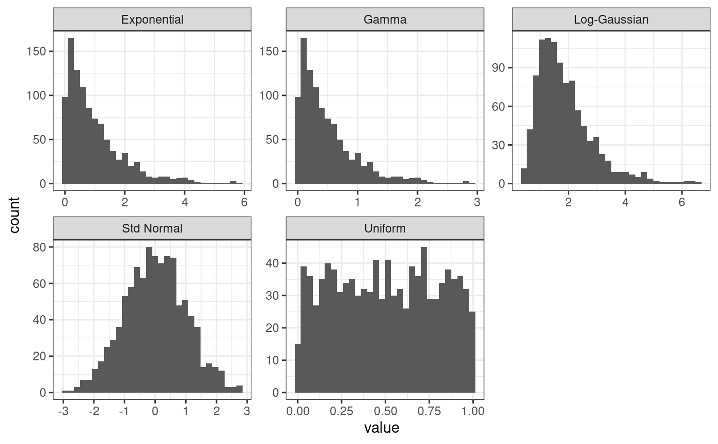idth`.

The package also provide inverse functions to retrieve the value of a parameter in the internal scale if the value in the ETAS scale is provided. Below an example

inv_gamma_t(gamma_t(1.2, 1, 2), 1, 2)
#> [1] 1.2
inv_unif_t(unif_t(1.2, 1, 2), 1, 2)
#> [1] 1.2
inv_exp_t(exp_t(1.2, 1), 1)
#> [1] 1.2
inv_loggaus_t(loggaus_t(1.2, 1, 2), 1, 2)
#> [1] 1.2

Once we have decided the priors that we are going to use in the analysis, we need to store the corresponding copula transformations in a list. The list one element for each parameter of the model ( $5$ ), and each element of the list must have name corresponding to the parameter. The names are fixed and should be mu, K, alpha, c_, and p. The parameter $c$ is referred as c_ to avoid clashing names with the R function c(). It is useful to do the same with the inverse functions also, this list will be used to set the initial value of the parameters later. The code below assumes that parameter $\mu$ has a Gamma distribution as prior with parameters $0.3$ and $0.6$ , parameters $K, \alpha,$ and $c$ have a Uniform prior on $(0,10)$ , while the parameter $p$ has a Uniform prior on $(1,10)$ .

# set copula transformations list
link.f <- list(
  mu = \(x) gamma_t(x, 0.3, 0.6),
  K = \(x) unif_t(x, 0, 10),
  alpha = \(x) unif_t(x, 0, 10),
  c_ = \(x) unif_t(x, 0, 10),
  p = \(x) unif_t(x, 1, 10)
)

# set inverse copula transformations list
inv.link.f <- list(
  mu = \(x) inv_gamma_t(x, 0.3, 0.6),
  K = \(x) inv_unif_t(x, 0, 10),
  alpha = \(x) inv_unif_t(x, 0, 10),
  c_ = \(x) inv_unif_t(x, 0, 10),
  p = \(x) inv_unif_t(x, 1, 10)
)

L’Aquila seismic sequence

Earthquake data is stored in the so-called earthquake catalogues. Many different catalogues exists for the same region and there is no easy way to decide which one is better. Here, we provide a subset of the HOmogenized instRUmental Seismic (HORUS) catalogue from 1960 to 2020. It can be downloaded from http://horus.bo.ingv.it/. See data-raw/horus.R for details on how the the subset was created from the original data set. This HORUS catalogue subset can be accessed directly using horus or ETAS.inlabru::horus:

# load HORUS catalogue
head(horus)
#>           time_string     lon     lat depth    M
#> 1 1960-01-03T20:19:34 15.3000 39.3000   290 6.34
#> 2 1960-01-04T09:20:00 13.1667 43.1333     0 3.94
#> 3 1960-01-06T15:17:34 12.7000 46.4833     4 4.69
#> 4 1960-01-06T15:20:53 12.7000 46.4667     0 4.14
#> 5 1960-01-06T15:31:00 12.7500 46.4333     0 3.00
#> 6 1960-01-06T15:45:00 12.7500 46.4333     0 3.00

Further documentation of the data set is available via ?horus.

The data reports for each earthquake the time as a string (time_string), longitude (lon) and latitude (lat) of the epicentre, the depth in kilometres (depth), and the moment magnitude (M).

To focus on the L’Aquila seismic sequence is sufficient to retain only the observations in a specific space-time-magnitude region that include the sequence of interest. For the L’Aquila sequence, we retain all the events with magnitude greater or equal than $2.5$ happened during 2009 with longitude in $(10.5, 16)$ and latitude in $(40.5, 45)$ . The L’Aquila sequence selected in this way should be composed by 1024 events. Any other seismic sequence can be selected similarly.

To do the selection is convenient to transform the time string in a Date object and to select the rows of the Horus catalogue verifying the conditions.

# transform time string in Date object
horus$time_date <- as.POSIXct(
  horus$time_string,
  format = "%Y-%m-%dT%H:%M:%OS"
)
# There may be some incorrectly registered data-times in the original data set,
# that as.POSIXct() can't convert, depending on the system.
# These should ideally be corrected, but for now, we just remove the rows that
# couldn't be converted.
horus <- na.omit(horus)

# set up parameters for selection
start.date <- as.POSIXct("2009-01-01T00:00:00", format = "%Y-%m-%dT%H:%M:%OS")
end.date <- as.POSIXct("2010-01-01T00:00:00", format = "%Y-%m-%dT%H:%M:%OS")
min.longitude <- 10.5
max.longitude <- 16
min.latitude <- 40.5
max.latitude <- 45
M0 <- 2.5

# set up conditions for selection
aquila.sel <- (horus$time_date >= start.date) &
  (horus$time_date < end.date) &
  (horus$lon >= min.longitude) &
  (horus$lon <= max.longitude) &
  (horus$lat >= min.latitude) &
  (horus$lat <= max.latitude) &
  (horus$M >= M0)

# select
aquila <- horus[aquila.sel, ]

The data can be visually represented by plotting the time of each event against the magnitude. This shows the clustering of the observations in correspondance of high magnitude events.

ggplot(aquila, aes(time_date, M)) +
  geom_point() +
  theme_bw()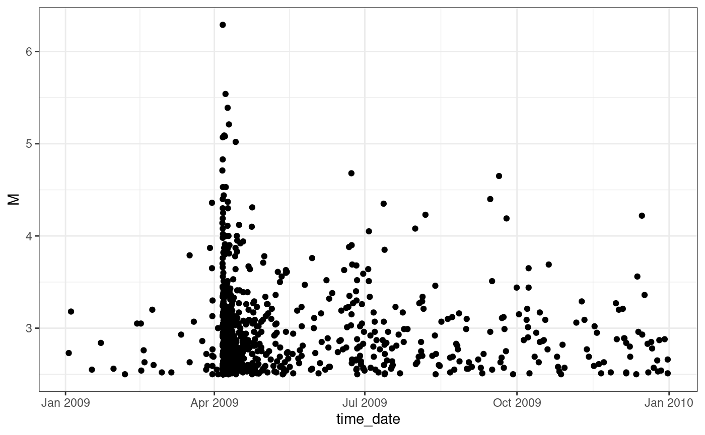

L’Aquila seismic sequence, times versus magnitudes

Data preparation to model fitting

We need to prepare a data.frame to be used as input data to fit the ETAS model. This data.frame must have three columns: ts for the time difference between the starting date and the occurrence time of the events (measured in days in this example), magnitudes for the magnitude of the events, and idx.p which is an index column with a different value for each event. The names are fixed and should not be changed

# set up data.frame for model fitting
aquila.bru <- data.frame(
  ts = as.numeric(
    difftime(aquila$time_date, start.date, units = "days")
  ),
  magnitudes = aquila$M,
  idx.p = 1:nrow(aquila)
)

After that, we need to set up the initial values of the parameters and the list containing the inlabru options to be used. The initial values should be stored in a list with elements th.mu, th.K, th.alpha, th.c, and th.p which corresponds to the ETAS parameters. The initial values must be provided in the internal scale and therefore it is useful to retrieve them using the inverse copula transformations that we set up before. In this way, we can find the values of the parameters in the internal scale given the value of the parameters in the ETAS scale. The example below uses $\mu = 0.5, K = 0.1, \alpha = 1, c = 0.1,$ and $p = 1.1$ as initial values. It is crucial to set initial values that do not cause numerical problems, in general this is achieved by setting initial values that are not nor from zero. The values provided below have worked well in various examples.

# set up list of initial values
th.init <- list(
  th.mu = inv.link.f$mu(0.5),
  th.K = inv.link.f$K(0.1),
  th.alpha = inv.link.f$alpha(1),
  th.c = inv.link.f$c_(0.1),
  th.p = inv.link.f$p(1.1)
)

Lastly, we need to set the list of inlabru options. The main elements of the list are :

bru_verbose: number indicating the type of diagnostic output. Set it to 0 for no output.
bru_max_iter: maximum number of iterations. If we do not set max_step the inlabru algorithm stops when the stopping criterion is met. However, setting max_step to values smaller than 1 forces the algorithm to run for exactly bru_max_iter iterations.
bru_method: for what is relevant here, the only thing that we may need to set is the max_step argument. If the algorithm does not converge without fixing a max_step then we suggest to try to fix it to some value below 1, in our experience $0.5$ or $0.2$ works well. In the example below the line setting bru_method is commented.
bru_initial: list of initial values created before.

# set up list of bru options
bru.opt.list <- list(
  bru_verbose = 3, # type of visual output
  bru_max_iter = 70, # maximum number of iterations
  # bru_method = list(max_step = 0.5),
  bru_initial = th.init # parameters' initial values
)

Note: In the option list, one can also set the number of threads allowed for INLA here, e.g. with num.threads = 8. This would override the global option that was set at the beginning of this tutorial. For code likely to be run on many different systems, using the global setting is easier to manage.

Model fitting

The function Temporal.ETAS fit the ETAS model and returns a bru object as output. The required inputs are:

total.data: data.frame containing the observed events. It have to be in the format described in the previous Section.
M0: cutoff magnitude. All the events in total.data must have magnitude greater or equal to this number.
T1: starting time of the time interval on which we want to fit the model.
T2: end time of the time interval on which we want to fit the model.
link.functions: list of copula transformation functions in the format described in previous sections.
coef.t., delta.t., N.max.: parameters of the temporal binning. The binning strategy is described in Appendix B of the paper Approximation of Bayesian Hawkes process with inlabru. The parameters corresponds to coef.t. $=\delta$ , delta.t. $=\Delta$ , and N.max. $=n_{\max}$ .
bru.opt: list of inlabru options as described in the previous Section.

# set starting and time of the time interval used for model fitting. In this case, we use the interval covered by the data.
T1 <- 0
T2 <- max(aquila.bru$ts) + 0.2 # Use max(..., na.rm = TRUE) if there may still be NAs here
# fit the model
aquila.fit <- Temporal.ETAS(
  total.data = aquila.bru,
  M0 = M0,
  T1 = T1,
  T2 = T2,
  link.functions = link.f,
  coef.t. = 1,
  delta.t. = 0.1,
  N.max. = 5,
  bru.opt = bru.opt.list
)
#> Start creating grid... 
#> Finished creating grid, time  1.823082

Create input list

After a model has been fitted the package ETAS.inlabru offers various functions to visually explore the output. They all require in input a list. The list must have different elements depending on the function we are going to use. To retrieve the posterior of the parameters and to sample from the posterior of the parameters we only need two elements:

model.fit: the output of Temporal.ETAS
link.functions: the list of copula transformations

# create input list to explore model output
input_list <- list(
  model.fit = aquila.fit,
  link.functions = link.f
)

Check marginal posterior distributions

The function get_posterior_param can be use to retrieve the marginal posteriors of the parameters in the ETAS scale. The function returns a list with elements:

post.df: a data.frame containing the posterior of the parameters. The data.frame has three columns, x with the value of the parameter, y with the corresponding value of the posterior, and param that indicates which ETAS parameter x and y are referring to.
post.plot: a ggplot object containing the plot of the marginal posteriors of the parameters

# get marginal posterior information
post.list <- get_posterior_param(input.list = input_list)

# plot marginal posteriors
post.list$post.plot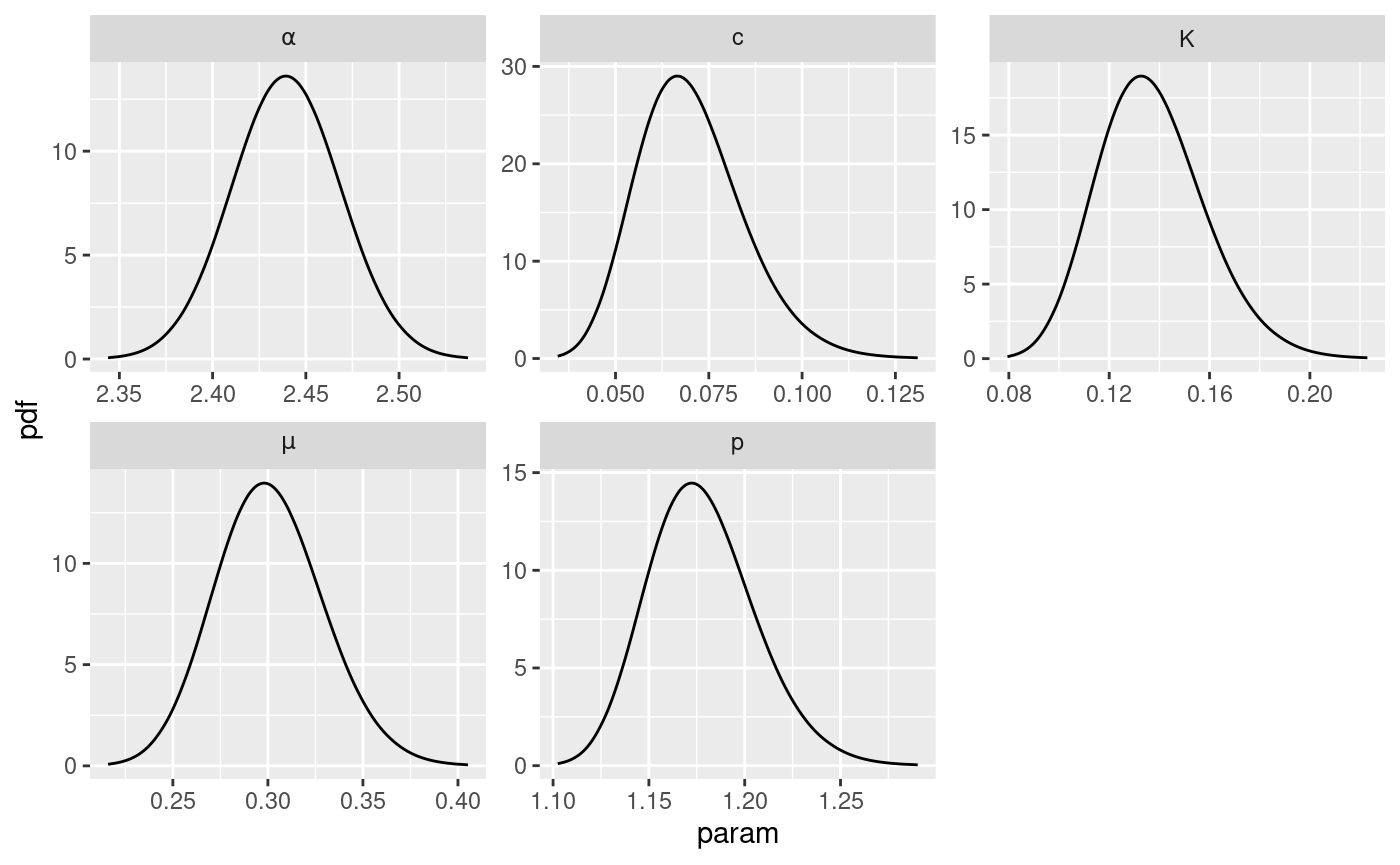

Sample the joint posterior and make pair plot

The function post_sampling generate samples from the joint posterior of ETAS parameters. The function takes in input:

input.list: a list with a model.fit element and a link.functions elements as described above.
n.samp: number of posterior samples.
max.batch: the number of posterior samples to be generated simultaneously. If n.samp $>$ max.batch, then, the samples are generated in parallel in batches of maximum size equal to max.batch. Default is $1000$ .
ncore: number of cores to be used in parallel when n.samp $>$ max.batch.

The function returns a data.frame with columns corresponding to the ETAS parameters

post.samp <- post_sampling(
  input.list = input_list,
  n.samp = 1000,
  max.batch = 1000,
  ncore = num.cores
)
#> Warning: The `ncore` argument of `post_sampling()` is deprecated as of ETAS.inlabru
#> 1.1.1.9001.
#> ℹ Please use future::plan(future::multisession, workers = ncore) in your code
#>   instead.
#> This warning is displayed once every 8 hours.
#> Call `lifecycle::last_lifecycle_warnings()` to see where this warning was
#> generated.

head(post.samp)
#>          mu         K    alpha          c        p
#> 1 0.3221930 0.1523066 2.513429 0.04218289 1.133595
#> 2 0.2997950 0.1483348 2.410908 0.07159829 1.185750
#> 3 0.2880364 0.1249349 2.478580 0.06221784 1.161846
#> 4 0.3281058 0.1350934 2.453335 0.07208162 1.196780
#> 5 0.2948586 0.1337900 2.431214 0.07597520 1.199861
#> 6 0.2601195 0.1401241 2.446638 0.06193619 1.160302

The posterior samples can be used to analyse the correlation between parameters. The function post_pairs_plot generate a pair plot of the posterior samples taken as input. The function has 4 arguments but they do not need to be all specified. The input are:

post.samp: data.frame of samples from the joint posterior distribution of the parameters. If it is NULL than the samples are generated by the function itself.
input.list: an input list with arguments model.fit and link.functions to be used to generate the posterior samples. This is used only if post.samp = NULL. Default is NULL.
n.samp: number of posterior samples. If it is NULL, then the samples in post.samp are used. If post.samp is NULL, then n.samp samples are generated from the joint posterior. If both post.samp and n.samp are not NULL then n.samp samples are randomly (uniformly and with replacement) selected from post.samp. Default is NULL
max.batch the number of posterior samples to be generated simultaneously. Same as before and only used when post.samp is NULL. Default is NULL

The function returns a list with two elements: post.samp with the posterior samples, and pair.plot which is a ggplot object containing the pair plot.

pair.plot <- post_pairs_plot(
  post.samp = post.samp,
  input.list = NULL,
  n.samp = NULL,
  max.batch = 1000
)
#> Registered S3 method overwritten by 'GGally':
#>   method from   
#>   +.gg   ggplot2
pair.plot$pair.plot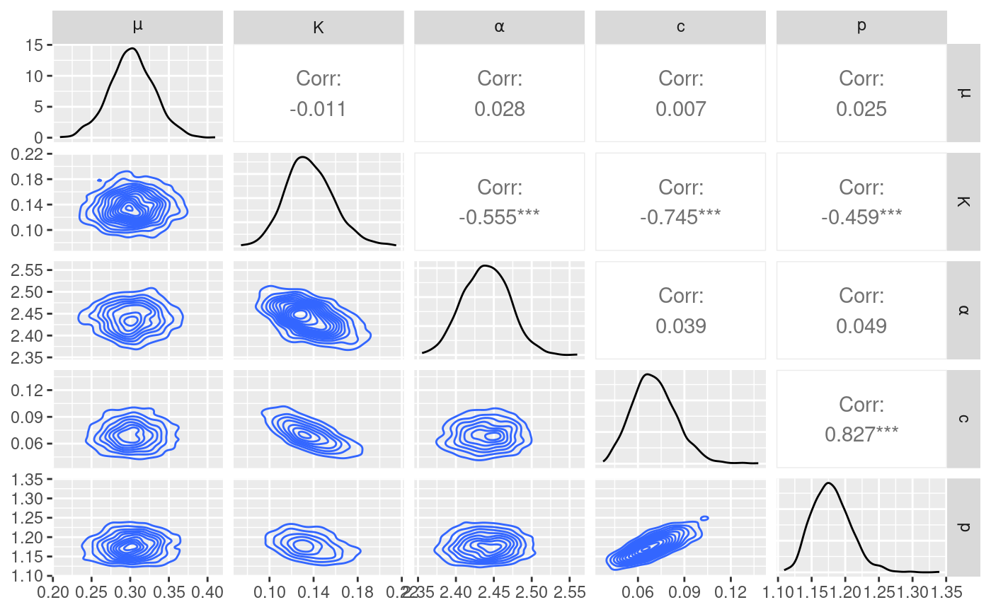

Check posterior number of events

A quantity of interest is the posterior distribution of the number of events. This can be accessed using the function get_posterior_N which requires as only input a list. However, the list needs to have some additional elements with respect the one used until now. Specifically, we need to add T12 with the extremes of the time interval of which we want to calculate the number of events, M0 the cutoff magnitude, and catalog.bru a data.frame containing the observed events. The latter has to be in the same format as total.data used for the Temporal.ETAS function.

The function returns a list of three elements: post.plot with a plot of the distribution, post.plot.shaded with a plot of the distribution with shaded regions representing $95\%$ interval for the distribution, and post.df with the data.frame used to generate the plots. The vertical line in the plots represent the number of events in the catalog.bru element of the input list.

# set additional elements of the list
input_list$T12 <- c(T1, T2)
input_list$M0 <- M0
input_list$catalog.bru <- aquila.bru

N.post <- get_posterior_N(input.list = input_list)
N.post$post.plot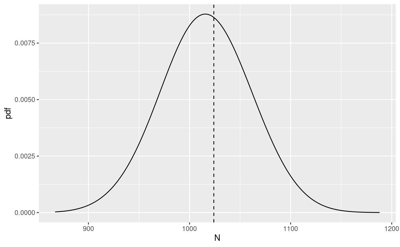

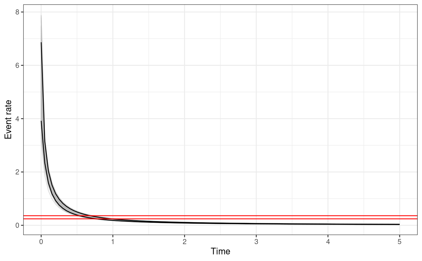
Posterior of the triggering function and Omori law

The functions triggering_fun_plot and triggering_fun_plot_prior plot, respectively, the quantiles of the posterior and prior distribution of the triggering function $g(t-t_h, mh)$ , namely,

$g(t - t_h, m_h) = K\exp\{\alpha(m_h - M_0)\}\left(\frac{t - t_h}{c} + 1\right)^{-p}$ The function takes in input

input.list: the input list as defined for the functions used previously.
post.samp: a data.frame of samples from the posterior distribution of the parameters. If it is NULL, then n.samp samples are generated from the posterior.
n.samp: number of posterior samples of the parameters to be used or generated.
magnitude: the magnitude of the event ( $m_h$ ).
t.end: the maximum value of $t$ for the plot.
n.breaks: the number of breaks in which the interval $(0, \texttt{t.end})$ is divided.

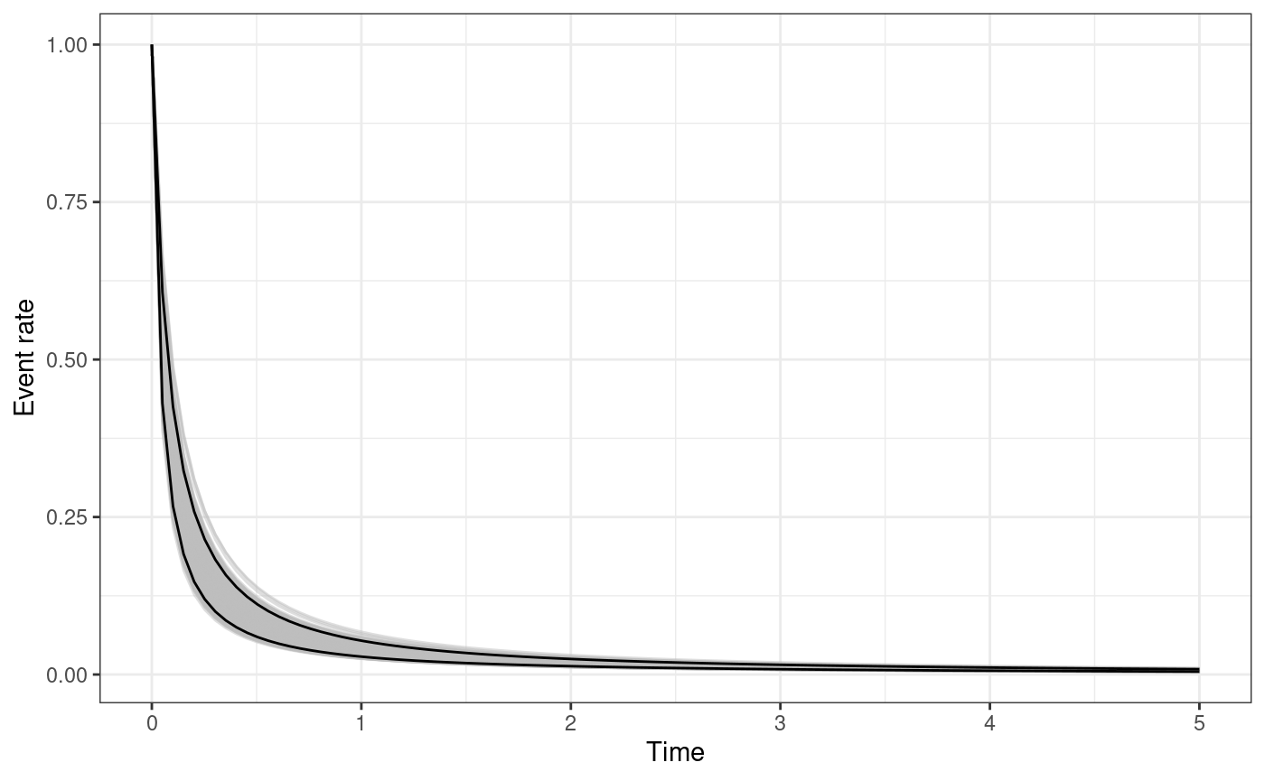
The function returns a ggplot object. For each sample of the parameters the triggering function between $0$ and t.end is calculated. The black solid lines represents the $95\%$ posterior interval of the function, the grey lines represent the triggering function calculated with the posterior samples, and the horizontal red lines represent the $95\%$ posterior interval of the background rate $\mu$ .

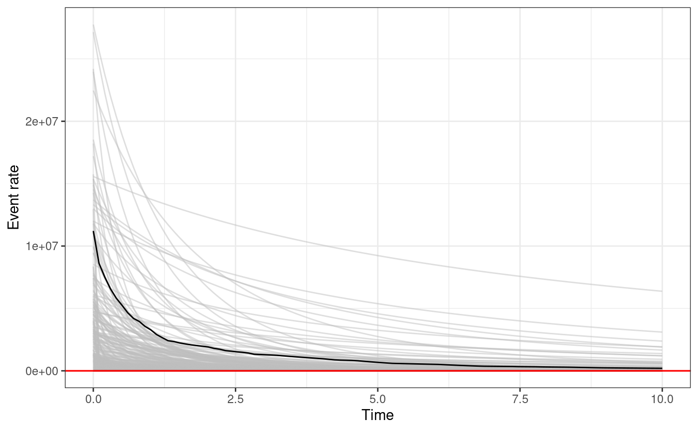
The function triggering_fun_plot_prior does the same but the value of the parameters are sampled according to the prior distribution rather than the posterior, and therefore, we do not need to specify a posterior samples data.frame.

triggering_fun_plot(
  input.list = input_list,
  post.samp = post.samp,
  n.samp = NULL, magnitude = 4,
  t.end = 5, n.breaks = 100
)

triggering_fun_plot_prior(input.list = input_list, magnitude = 4, n.samp = 1000, t.end = 10)

The functions omori_plot_posterior and omori_plot_prior do the same as the functions triggering_fun_plot and triggering_fun_plot_prior but considering only

$\left(\frac{t- t_h}{c} + 1\right)^{-p}$ instead of the whole triggering function and without the background rate.

omori_plot_posterior(input.list = input_list, post.samp = post.samp, n.samp = NULL, t.end = 5)

omori_plot_prior(input.list = input_list, n.samp = 1000, t.end = 5)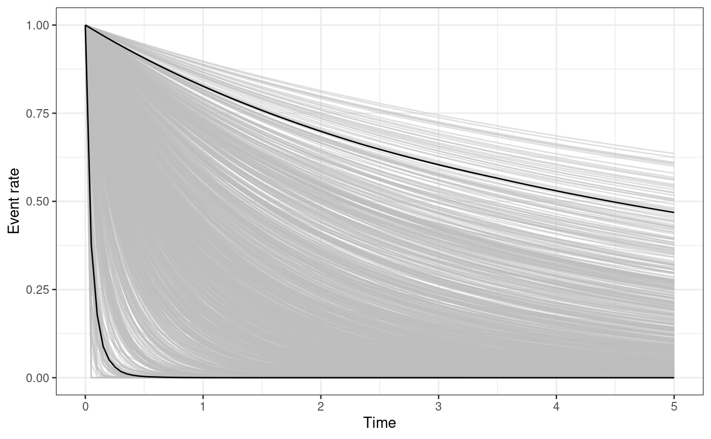

Generate synthetic catalogues from model

An earthquake forecast is usually composed by a collection of synthetic catalogues from a model. The package ETAS.inlabru provides a function to generate synthetic catalogues for a given set of parameters. This can be used both to produce forecasts or to simply produce synthetic catalogues. The function to generate synthetic catalogues is called generate_temporal_ETAS_synthetic which takes as input

theta: a list of ETAS parameters with names mu, K, alpha, c, and p, corresponding to the ETAS parameters.
beta.p: the parameter of the magnitude distribution
M0: cutoff magnitude, all the generated event will have magnitude greater than M0.
T1: starting time of the catalogue (the unit of measure depends on the unit used to fit the model).
T2: end time of the catalogue (the unit of measure depends on the unit used to fit the model).
Ht: set of known events. They can also be between T1 and T2, this is useful when we want to generate catalogues with imposed events.

Regarding the magnitude distribution, it is an exponential, specificically we assume

$m - M_0 \sim \text{Exp}(\beta)$ The parameter $\beta$ is usually estimated independently from the ETAS parameters. We use the maximum likelihood estimator for $\beta$ which is given by

$\hat\beta = \frac{1}{\bar{m} - M_0}$ where $\bar m$ is the mean of the observed magnitudes values.

# maximum likelihood estimator for beta
beta.p <- 1 / (mean(aquila.bru$magnitudes) - M0)

The function returns a list of data.frame, each element of the output list corresponds to a different generation. The data.frame have three columns: occurence time (ts), magnitude (magnitudes), a the generation identifier (gen). The generation identifier uses the following convention, $-1$ indicates the events in Ht with time between T1 and T2, $0$ indicates the first generation offspring of the events with gen equal $-1$ , $1$ indicates background events, $2$ all the offspring of the events with gen equal $0$ or $1$ , $3$ indicates all the offspring of the events with gen equal $2$ , $4$ indicates all the offspring of the events with gen equal $3$ , and so on. To obtain a unique data.frame containing all the simulated events it is sufficient to bind by rows all the generations.

Below an example in which we generate 1 synthetic catalogue using as parameters one of the posterior samples generated before. The catalogue covers the same time span as the L’Aquila catalogue and we impose the greatest event in the sequence.

synth.cat.list <- generate_temporal_ETAS_synthetic(
  theta = post.samp[1, ], # ETAS parameters
  beta.p = beta.p, # magnitude distribution parameter
  M0 = M0, # cutoff magnitude
  T1 = T1, # starting time
  T2 = T2, # end time
  Ht = aquila.bru[which.max(aquila.bru$magnitudes), ] # known events
)
# merge into unique data.frame
synth.cat.df <- do.call(rbind, synth.cat.list)
# order events by time
synth.cat.df <- synth.cat.df[order(synth.cat.df$ts), ]

ggplot(synth.cat.df, aes(ts, magnitudes, color = as.factor(gen))) +
  geom_point(size = 0.5)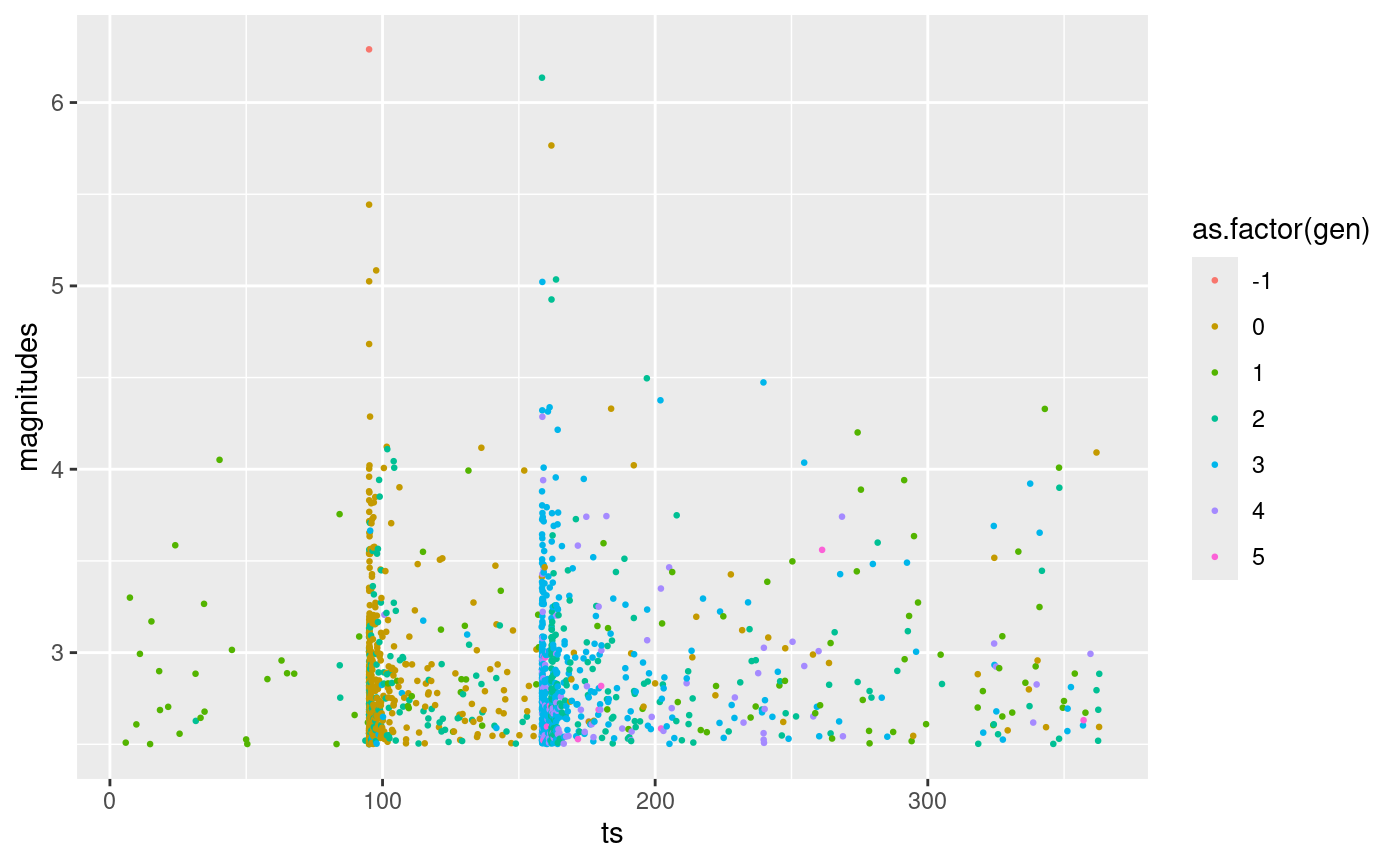

We can easily generate multiple catalogues. The code below generates 8 catalogues using different samples from the posterior distribution of the parameters. The red point indicates the event that we have imposed and the last panel represents the observed L’Aquila sequence.

set.seed(2)
n.cat <- 8
# generate catalogues as list of lists
multi.synth.cat.list <- lapply(seq_len(n.cat), \(x)
generate_temporal_ETAS_synthetic(
  theta = post.samp[x, ],
  beta.p = beta.p,
  M0 = M0,
  T1 = T1,
  T2 = T2,
  Ht = aquila.bru[which.max(aquila.bru$magnitudes), ]
))

# store catalogues as list of data.frames
multi.synth.cat.list.df <- lapply(multi.synth.cat.list, \(x) do.call(rbind, x))
# set catalogue identifier
multi.synth.cat.list.df <- lapply(seq_len(n.cat), \(x) cbind(multi.synth.cat.list.df[[x]],
  cat.idx = x
))
# merge catalogues in unique data.frame
multi.synth.cat.df <- do.call(rbind, multi.synth.cat.list.df)

# we need to bing the synthetics with the observed catalogue for plotting
cat.df.for.plotting <- rbind(
  multi.synth.cat.df,
  cbind(aquila.bru[, c("ts", "magnitudes")],
    gen = NA,
    cat.idx = "observed"
  )
)

# plot them
ggplot(cat.df.for.plotting, aes(ts, magnitudes)) +
  geom_point(size = 0.5) +
  geom_point(
    data = aquila.bru[which.max(aquila.bru$magnitudes), ],
    mapping = aes(ts, magnitudes),
    color = "red"
  ) +
  facet_wrap(facets = ~cat.idx)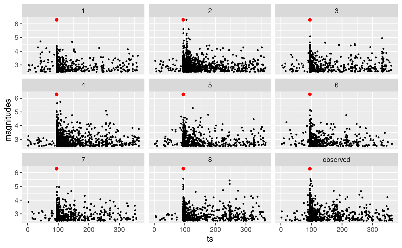

Forecasting

An earthquake forecast is usually collection of synthetic catalogues generated from a model. For bayesian models we can reflect the uncertainty on the parameters values by generating each synthetic catalogue composing the forecast using a different set of parameters sampled from the join posterior distribution. We can generate forecasts using the function Temporal.ETAS.forecast. The function takes as input

post.samp: a data.frame of samples from the posterior distribution of the parameters with the same format described in previous sections.
n.cat: the number of synthetic catalogues composing the forecast. If n.cat is greater than nrow(post.samp), then the rows of post.samp are sampled uniformly and with replacement n.cat times. If n.cat is smaller than nrow(post.samp), then, then the rows of post.samp are sampled uniformly and without replacement n.cat times. If n.cat is NULL or equal to nrow(post.samp), then, post.samp is used as it is.
ncore: the number of cores to be used to generate the synthetic catalogues in parallel.

The remaining inputs (beta.p, M0, T1, T2, Ht) are the same as the ones used in generate_temporal_ETAS_synthetic.

The output of the function is a list with two elements: fore.df and n.cat. The element fore.df is a data.frame with the synthetic catalogues binded together by row, it is the same as multi.synth.cat.df created before. The element n.cat is just the number of catalogues generated. We need n.cat because zero-events catalogues do not appear in fore.df, and the corresponding cat.idx value is missing. Therefore we need n.cat to recover the total number of catalogues.

The code below creates a daily forecast for the 24 hours starting 1 minute after the event with the greatest magnitude in the sequence. The starting date and end date of the forecast are expressed in the same unit used in the catalogue to fit the model (days in this case). Day zero correspond to start.date stated in the beginning of the document which for the example is $2009-01-01 00:00:00$ . The forecast is generated assuming known all the events in the catalogue occurred before the forecasting period.

# express 1 minute in days
min.in.days <- 1 / (24 * 60)
# find time of the event with the greatest magnitude
t.max.mag <- aquila.bru$ts[which.max(aquila.bru$magnitudes)]
# set starting time of the forecasting period
T1.fore <- t.max.mag + min.in.days
# set forecast length
fore.length <- 1
# set end time of the forecasting period
T2.fore <- T1.fore + fore.length
# set known data
Ht.fore <- aquila.bru[aquila.bru$ts < T1.fore, ]

# produce forecast
daily.fore <- Temporal.ETAS.forecast(
  post.samp = post.samp, # ETAS parameters posterior samples
  n.cat = nrow(post.samp), # number of synthetic catalogues
  beta.p = beta.p, # magnitude distribution parameter
  M0 = M0, # cutoff magnitude
  T1 = T1.fore, # forecast starting time
  T2 = T2.fore, # forecast end time
  Ht = Ht.fore, # known events
  ncore = num.cores
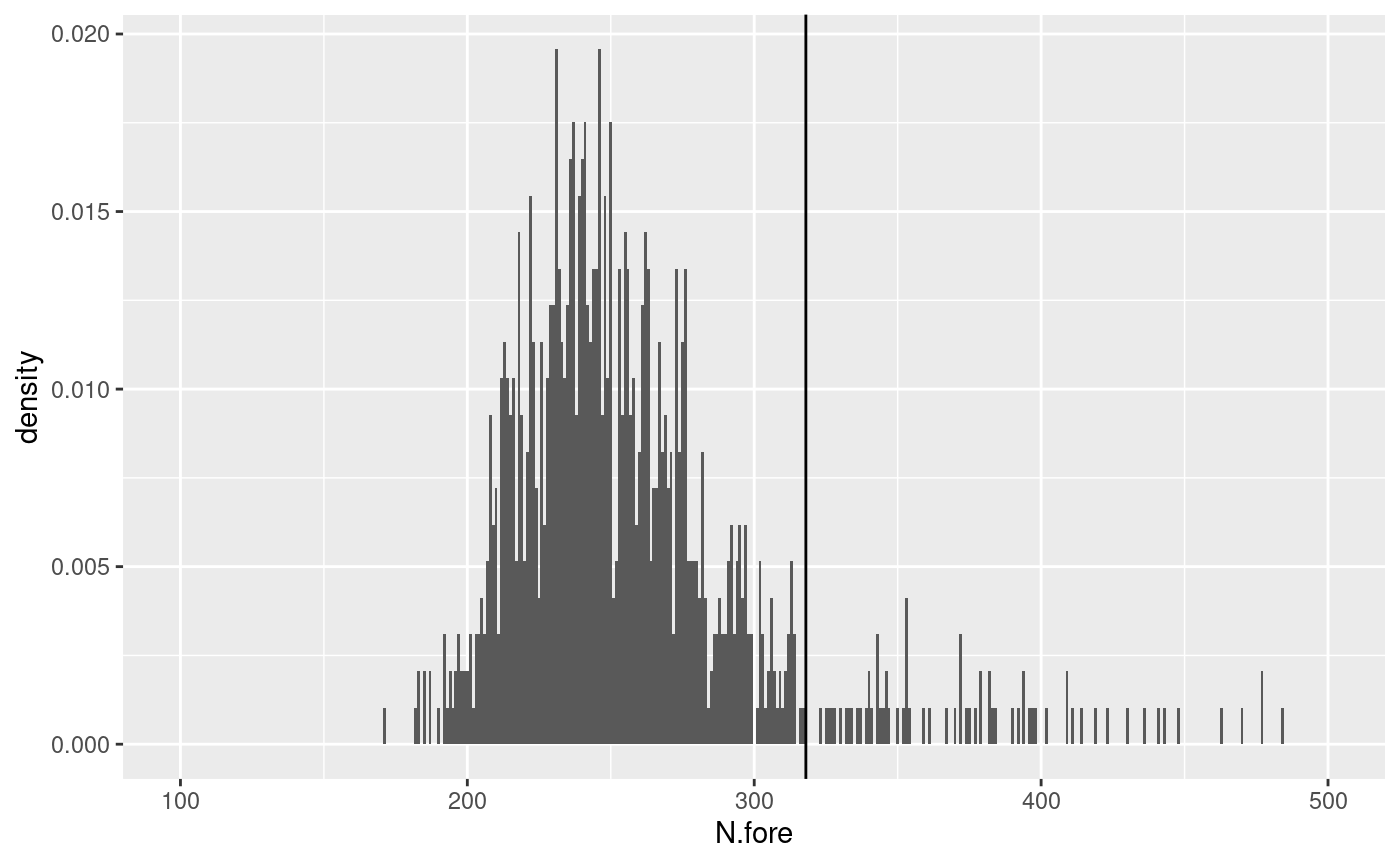
) # number of cores

We can easily retrieve the predictive distribution of the number of events in the forecasting period looking at the frequencies with which the catalogue identifiers appears in the fore.df element. Indeed, the number of rows of fore.df with the same cat.idx value represents the number of events in that synthetic catalogue. So, if the frequency with which each catalogue identifier appears in fore.df$cat.idx correspond to the number of events in that catalogue. This allows to easily retrieve the predictive distribution of the number of events using the code below. We remark that in this case we can not use the function table to find the frequencies of elements of fore.df$cat.idx. This is because the catalogue identifier of zero-events catalogues are not present in fore.df$cat.idx. So using table would lead to have zero probability of having zero events in a day, quantity that is crucial if we are intersted in the probability of earthquake activity (probability of having at least one event).

# find number of events per catalogue
N.fore <- vapply(
  seq_len(daily.fore$n.cat),
  \(x) sum(daily.fore$fore.df$cat.idx == x), 0
)
# find number of observed events in the forecasting period
N.obs <- sum(aquila.bru$ts >= T1.fore & aquila.bru$ts <= T2.fore)
# plot the distribution
ggplot() +
  geom_histogram(aes(x = N.fore, y = after_stat(density)), binwidth = 1) +
  geom_vline(xintercept = N.obs) +
  xlim(100, 500)
#> Warning: Removed 29 rows containing non-finite outside the scale range
#> (`stat_bin()`).
#> Warning: Removed 2 rows containing missing values or values outside the scale range
#> (`geom_bar()`).

Francesco Serafini

2023-06-27