2a Temporal Model: Generating synthetic temporal ETAS catalogues

library(ETAS.inlabru)
library(ggplot2)
library(dplyr)
library(magrittr)
# library(tidyquant)

# Increase/decrease num.cores if you have more/fewer cores on your computer.
# future::multisession works on both Windows, MacOS, and Linux
num.cores <- 2
future::plan(future::multisession, workers = num.cores)
INLA::inla.setOption(num.threads = num.cores)
# To deactivate parallelism, run
#   future::plan(future::sequential)
#   INLA::inla.setOption(num.threads = 1)

Create catalogue

• define ETAS parameters
• define model domain
• specify a history
• generate ETAS sample
• plot the results

mu <- 1070. / 365
K <- 0.089
alpha <- 2.29
c <- 0.011
p <- 1.08

modelledDuration <- 10 # [days]

M0 <- 2

theta_etas <- data.frame(mu = mu, K = K, alpha = alpha, c = c, p = p)

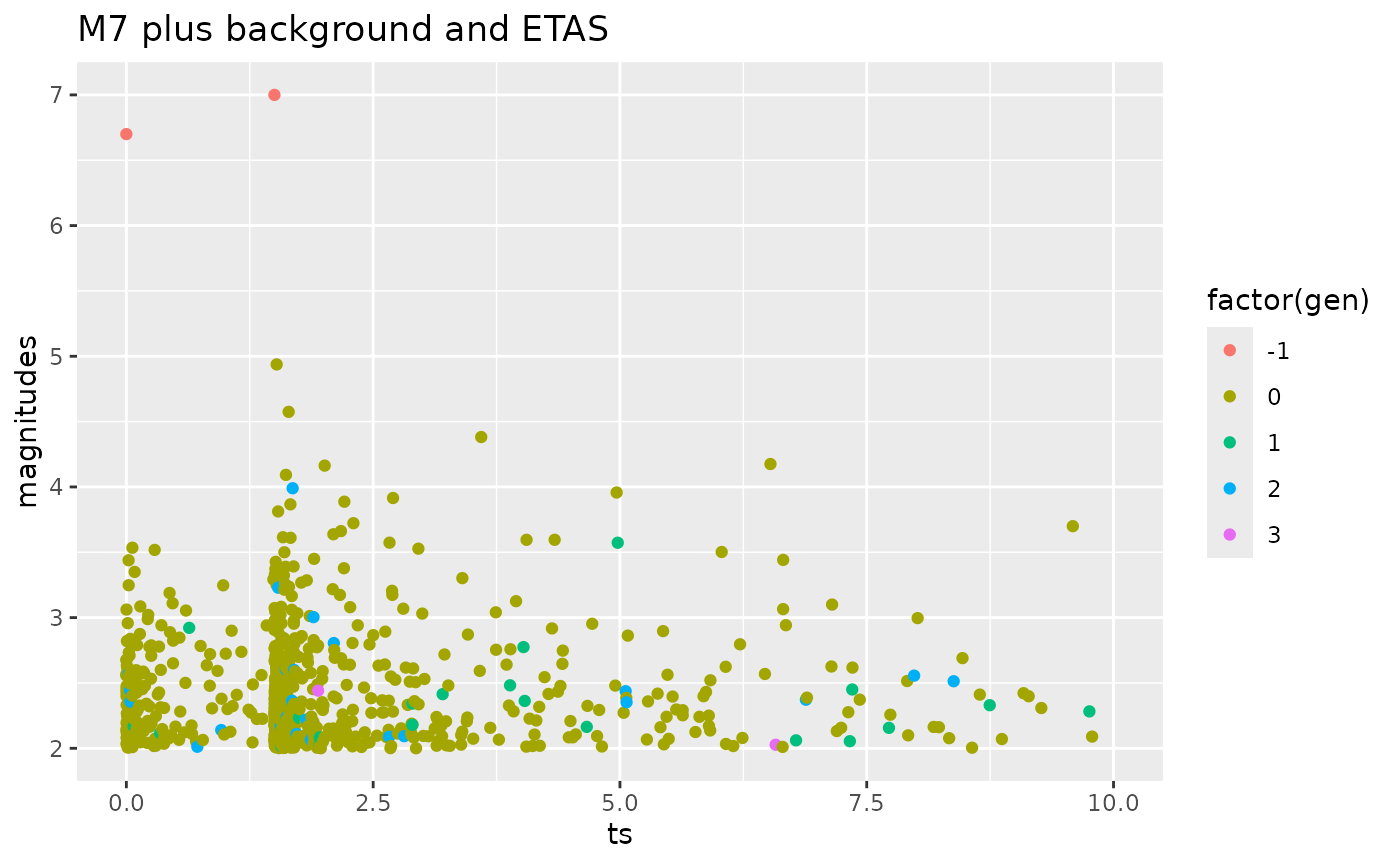
Ht <- data.frame(ts = c(0., 1.5), magnitudes = c(6.7, 7.))

combined.M7.ETAS.cat <-
  generate_temporal_ETAS_synthetic(
    theta = theta_etas,
    beta.p = log(10),
    M0 = M0,
    T1 = 0,
    T2 = modelledDuration,
    Ht = Ht,
    format = "df"
  )
combined.M7.ETAS.cat$ID <- seq_len(nrow(combined.M7.ETAS.cat))

ggplot(combined.M7.ETAS.cat) +
  geom_point(aes(x = ts, y = magnitudes, color = factor(gen))) +
  xlim(0, modelledDuration) +
  ggtitle("M7 plus background and ETAS")

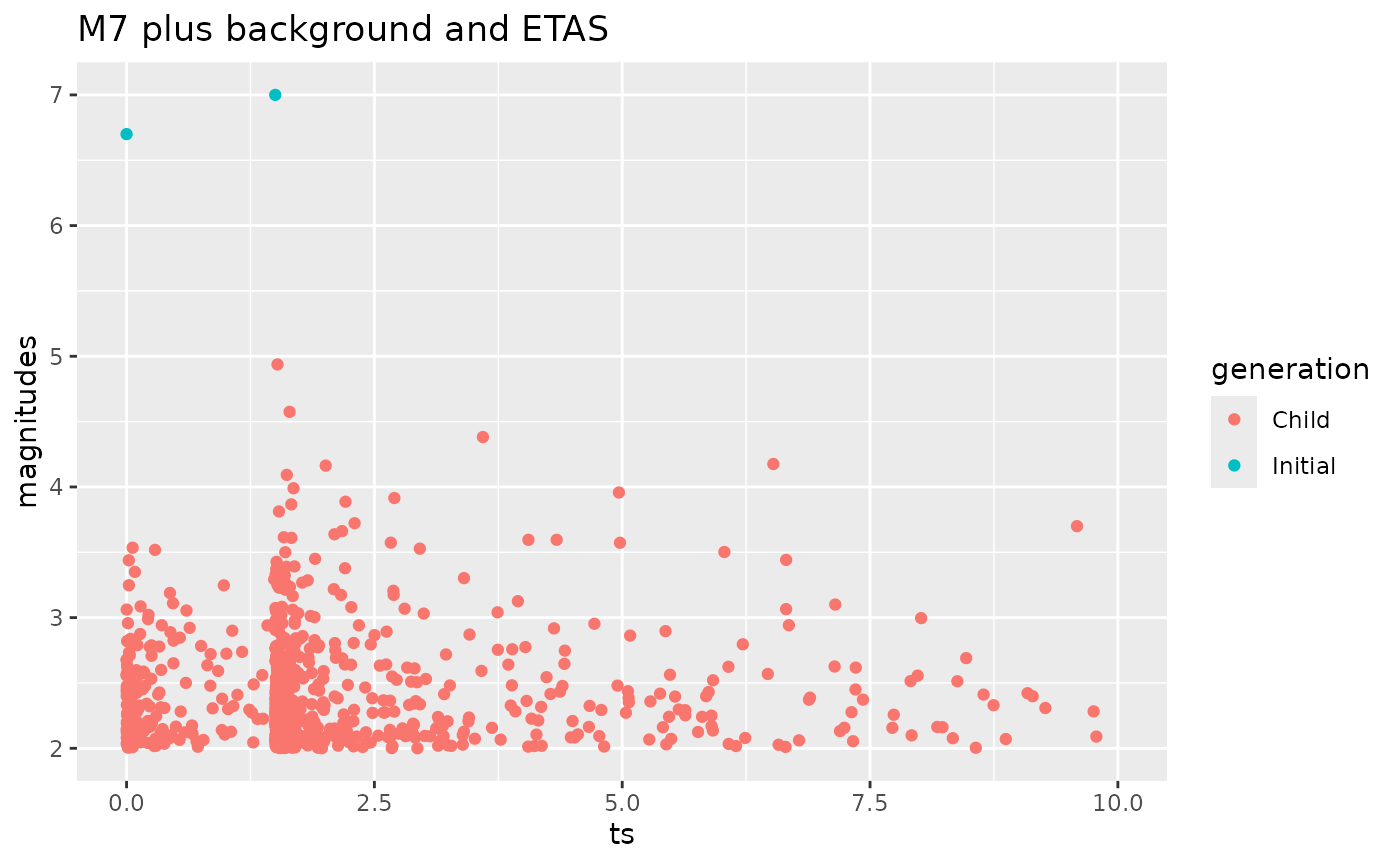
ggplot(combined.M7.ETAS.cat %>%
  mutate(generation = if_else(gen == -1, "Initial", "Child"))) +
  geom_point(aes(x = ts, y = magnitudes, color = generation)) +
  xlim(0, modelledDuration) +
  ggtitle("M7 plus background and ETAS")

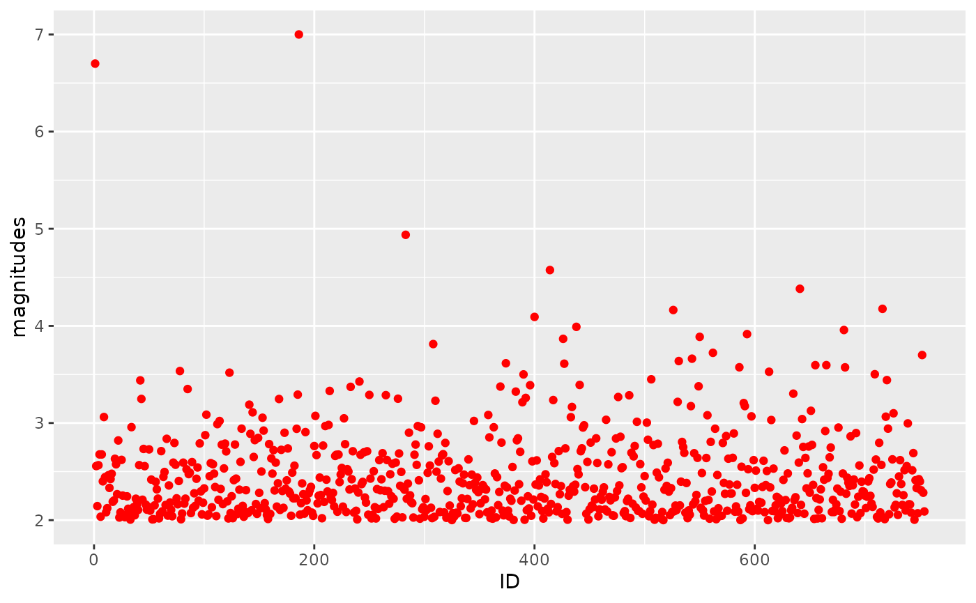
ggplot() +
  geom_point(data = combined.M7.ETAS.cat, aes(x = ID, y = magnitudes), color = "red") #+

#  geom_ma(data = combined.M7.ETAS.cat, aes(x=ID, y=magnitudes), ma_fun = SMA, n = 10)